|
|
|


Creating data
subsets by applying filters
Statistical
Functions on Plotted Data
Introduction
VOPlot 3D (VOTable 3D Plotting tool) is an applet for plotting different astronomical graphs using data stored in VOTable format. It supports different operations such as rotation, panning and zooming on the plot. VOPlot is available in desktop and web-based version.
Click here for Release Notes and disclaimer information.
About VOPlot
VOPlot 3D has been developed as a part of the Virtual Observatory - India initiative by Persistent Systems and the Inter-University Centre for Astronomy and Astrophysics (IUCAA). The VO-India project is supported by the Ministry of Information and Communication Technology of the Government of India.
VOPlot 3D uses Java 3D API (v1.3.1) for plotting different astronomical graphs in three-dimension. Java 3D is a standard extension to the Java 2 JDK. It is an interface for writing programs to display and interact with three-dimensional graphics.
3rd Party Tools implemented:
· SAVOT (Simple Access to VOTable): VOPlot 3D uses SAVOT (Simple Access to VOTable) to read VOTable documents.
· Colt: VOPlot 3D uses Colt libraries from CERN for statistical calculations of the VOTable data.
· Ptplot (v5.2): VOPlot 3D uses Ptplot (v5.2) for display of Box Plot.
Getting Started
Standalone Version:
* To use the standalone version of VOPlot, you will need to download the executable jar file named voplot3D.jar. The file can be executed by typing the following command at the command prompt:
|
java -jar voplot3d.jar |
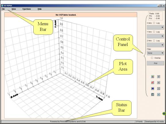
This will open a java application window as shown in the Figure 0.
To use data from a VOTable you will need to load it first. You can specify the path of a VOTable on your personal computer (PC) by clicking on the "Open" submenu from the "File" menu. The message on the status bar will indicate whether the file was loaded successfully or not.
* To see the version of JRE installed, type the following command at the command prompt:
|
java –version |
* To increase the memory of JVM to 64 Mb, type the following command at the command prompt:
|
java –Xms64m -jar voplot3d.jar |
Click here for installation instructions for Java 3D API.
Note: To run VOPlot 3D version1.0, you must have Java Runtime Environment (1.4 or later), Java 3D API (1.3.1) OpenGL 1.1 or DirectX (8.0 or later) is required.
Loading Data In VOPlot 3D:
Currently VOPlot3D uses data in VOTable format for plotting. The default columns for the graph are loaded on the basis of FIELD UCDs. Once the table is loaded, the metadata of the VOTable is read and the numeric columns are retrieved and listed in the combo boxes for X, Y and Z-axis on the control panel.
Figure 0
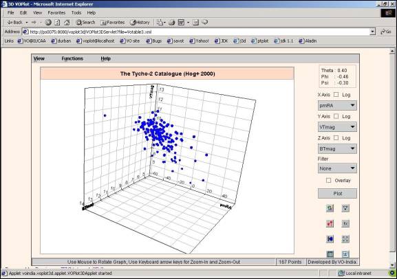
Web Version:
In the Web-based version of VOPlot 3D, the
VOTable is loaded automatically from the web server.
Figure 1
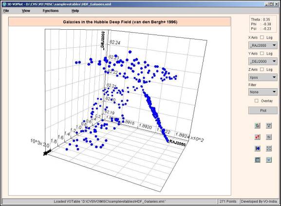
Plotting Scatter Plots
To draw a plot of one columns against the other,
- Select the column to be plotted on the X-axis.
- Select the column to be plotted on the Y-axis.
- Select the column to be plotted on the Z-axis.
- Click "Plot" button.
You can see the scatter plot. If required, you can plot data points on a log scale by setting the option appropriately using the "Log" checkbox.
Figure 2
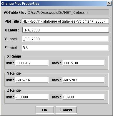
Changing Plot properties
To change the plot properties click on the " View -> Plot Properties" menu, which opens the "Change Plot Properties" dialog as shown in Figure 3.
The various plot properties such as Title of the plot, X-axis label, Y-axis label, Z-axis label, X-axis range, Y-axis range and Z-axis range can be changed.
Figure 3
Zooming And Panning
Following keys can be used for zooming and panning of the plot.
|
Sr. No. |
Key |
|
Effect |
|
1. |
Up Arrow key |
|
To zoom out of the graph |
|
2. |
Down Arrow key |
|
To zoom in to the graph |
|
3. |
Home Key |
Home
|
Reset graph to the centre |
|
4. |
Left Arrow Key |
|
For left lateral translation |
|
5. |
Right Arrow Key |
|
For right lateral translation |
|
6. |
Page Up Key |
PgUp
|
To move the graph up |
|
7. |
Page Down Key |
PgDn |
To move the graph down |
Note: Zooming-In and Zooming-Out of the graph is restricted up to a certain depth.
Plot Rotation
To rotate the Plot in any direction, press the left mouse button on the graph and move it in required direction of rotation. On rotation of the graph, the corresponding euler angles (theta, phi and psi) are displayed in radians on the top right-hand corner on the control panel.
Euler angles’ panel is shown in Figure 4 below.
Figure 4
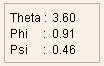
Displaying Euler Angles
The plot in 3D VOPlot can be rotated about X, Y or Z-axis using the mouse to get any desired projection. The amount of rotation involved (change in the ‘line of sight’) is represented in terms of Euler angles, Θ (theta), Φ (phi), Ψ (psi), which are angles of rotation about the X, Y and Z-axes in that order. Corresponding Euler angles for any projection are displayed on the upper-right corner on the control panel as shown in Figure 4 above.
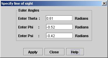
It is possible to get the projection of the plot by providing the corresponding Euler angles as well. For this, the Euler angles can be specified in ‘Specify line of sight’ dialog under View->Enter Line of Sight as shown in Figure 5 below.
Figure 5
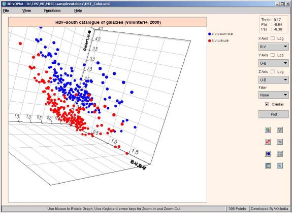
Overlaying Plots
To overlay plots (simultaneously viewing multiple plots with similar range on the same axes system)
- Select column to be plotted on the X-axis.
- Select column to be plotted on the Y-axis.
- Select column to be plotted on the Z-axis.
- Click "Plot" button.
- Select column to be plotted on X-axis (represents another plot).
- Select column to be plotted on Y-axis (represents another plot)
- Select column to be plotted on Z-axis (represents another plot)
- Set the "Overlay" option.
- Click "Plot" button.
You can see the second plot overlaid on the first one if the second one is in the same range as the previous one. Only that portion of the second plot is visible that is within the already plotted range.
To see the entire range of
points, click on the ‘Show full range of data’ button ( ![]() ) in the toolbar on
control panel. To reset the plot to the previous range, click on the ‘Reset
axis ranges’ button (
) in the toolbar on
control panel. To reset the plot to the previous range, click on the ‘Reset
axis ranges’ button (![]() ).
).
A screen shot of overlaid plots can be seen in Figure 6 below.
Figure 6
A different marker color will be used for each plot, to allow one to differentiate between the plots. Currently 16 datasets can be overlaid.
Transformations on columns
One can create new columns by defining transformations on them. You can use expressions with arithmetic operators, trigonometric functions, and miscellaneous functions shown below to create new columns. You can use transformed columns for plotting.
Operators Allowed
|
+ |
Addition |
|
- |
Subtraction |
|
* |
Multiplication |
|
/ |
Division |
Functions
|
log(a) |
Log to the base 10. |
|
ln(a) |
Natural Log of "a" with base e, where e is Euler's number (i.e. 2.718...). |
|
pow(a,b) |
"a" raised to power of "b". |
|
sqrt(a) |
Square root of "a". |
|
exp(a) |
Returns the exponential number e (i.e. 2.718...) raised to the power of "a". |
|
dexp(a) |
10 raised to the power of "a". |
|
cos(a) |
Trigonometric cosine of an angle. a = an angle in radians. |
|
acos(a) |
Computes the arc cosine of "a". "a" must range from -1 to 1; the resulting angle is in radians and will range from 0 to pi. |
|
sin(a) |
Trigonometric sine of an angle. a = an angle in radians. |
|
asin(a) |
Computes the arc sine of "a". "a" must range from -1 to 1; the resulting angle is in radians and will range from -pi/2 to pi/2. |
|
tan(a) |
Trigonometric tangent of an angle. a = an angle in radians. |
|
atan(a) |
Computes the arc tangent of "a". The resulting angle is in radians and will range from -pi/2 to pi/2. |
|
toradians(a) |
Converts an angle measured in degrees to an equivalent angle measured in radians. |
|
todegrees(a) |
Converts an angle measured in radians to an equivalent angle measured in degrees. |
Creating new columns
- To define transformations on columns click on "Create new columns" submenu from the "Functions" menu to display the "Create new columns" Dialog Box.
- In the "Create new virtual columns" Dialog Box, you can see the column names, UCD and their Id (used for expression building) and the expression with which they were created.
- For creating a new column, type in the new column name (example col2) and the expression using the functions shown above. Example: $4+log($6). Add a unit as well for the new column (Optional).
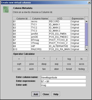
- The expression can also be formed with the help of "Operator Calculator" as shown in Figure 7. When you click on a row present in the "Column Metadata" table, then the corresponding Column Id appears in the text box for "Enter expression". By clicking on any of the buttons in the "Operator Calculator", the corresponding operator or function appears in the text box for "Enter expression". This feature eliminates the need of typing in the expression and allows automatic creation of the expression.
The dialog box for creating new columns is shown in Figure 7.
Figure 7
Creating data subsets by applying filters
You can create new data subsets by defining filters on them. You can use a condition with relational operators and logical operators with operators and functions shown above to create new data subsets. Data subsets can be used for plotting.
Operators Allowed
|
< |
Less than |
|
<= |
Less than or equal to |
|
> |
Greater than |
|
>= |
Greater than or equal to |
|
== |
Equal to |
|
!= |
Not equal to |
|
&& |
And |
|
|| |
Or |
|
! |
Not |
Creating new data subsets
- To define new data subsets on columns click on the "Create Filters" submenu from the "Functions" menu to display the "Create new data subsets" dialog box.
- In this dialog box, you can see the column names, UCD and their Id (used for expression building) and the expression with which they were created. You can also see the data subsets that you previously created with their names and conditions.
- For creating a new data subset, type in the new subset name (example f1Glat) and the filter definition using the functions and relational operators shown in table above. You can also make use for arithmetic operators and functions listed for "Transformations on columns". Example: $1 > 0 || ($3! = 0 && $2 > 100)
- The expression can also be formed with the help of "Operator Calculator" as shown in the following figure. When you click on a row present in the "Column Metadata" table, then the corresponding Column Id appears in the text box for "Enter expression". By clicking on any of the buttons in the "Operator Calculator", the corresponding operator or function appears in the text box for "Enter expression". This feature eliminates the need of typing in the expression and allows automatic creation of the expression.
The dialog box for creating data subsets is shown in Figure 8.
Figure 8
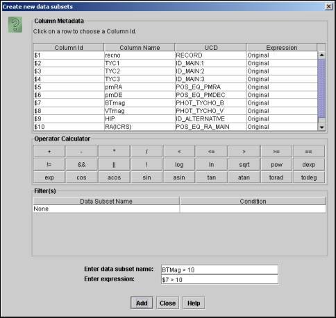
Once a data subset is created you can plot data from the subset. This can be done by choosing the data subset from the Filters combo box in the main applet window.
Note: "None" represents the complete data. Only data points satisfying the filter condition will be considered for plotting.
Statistical Functions on Plotted Data
Statistical functions can be applied on the plotted data.
Applying Statistical Functions
- To apply statistical functions, click on "Generate Statistics" submenu from the "Functions" menu. The "Plot Statistics" dialog box will open.
- You can choose the data subset from the filter combo box. Note: "None" represents the complete data.
- Select X, Y and Z axes and click "Calculate" button. Note: Default columns are picked up from the current plot. The results are displayed on the same window.
The dialog box is divided into two tabs – basic and advanced functions. The basic functions require only one data array, while the advanced functions require two or three data arrays as parameters.
The following statistical functions are currently supported.
|
Sr. No. |
Function name |
Input Columns |
|
1 |
Number of observations |
X |
|
2 |
Range |
X |
|
3 |
Minimum |
X |
|
4 |
Maximum |
X |
|
5 |
Mean |
X |
|
6 |
Variance |
X |
|
7 |
Standard deviation |
X |
|
8 |
Skew |
X |
|
9 |
Kurtosis |
X |
|
10 |
Linear correlation |
X, Y |
|
11 |
Significance (t) for Linear correlation |
X, Y |
|
12 |
Probability for Linear correlation |
X, Y |
|
13 |
Rank correlation |
X, Y |
|
14 |
Partial correlation |
X, Y, Z |
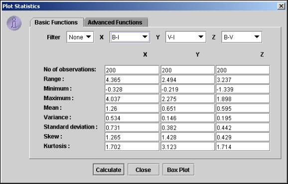
VOPlot takes the entire data range into consideration while evaluating the statistical functions. This will evaluate the statistical functions for the currently plotted columns, along with the applied filter, if any, in the current axes ranges. Sample dialog box with basic tab selected showing plot statistics is shown in Figure 9.
Figure 9
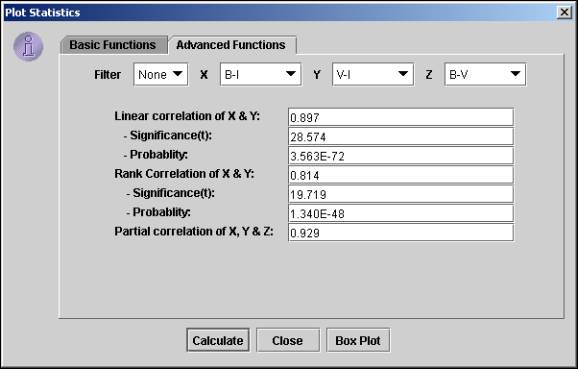
Sample "Advanced Functions" tab is shown in Figure 10.
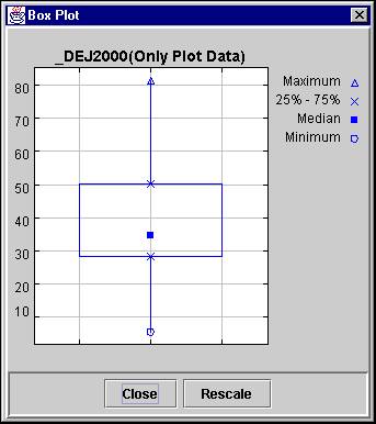
Displaying Box Plot
A Box plot provides an excellent visual summary of many important aspects of a distribution. It identifies the middle 50% of the data, the median and the extreme points.
Click on the "Box Plot" button on the "Plot statistics" dialog to display the Box Plot for the X column. Sample Box Plot is shown in Figure 11 below.
Figure 11
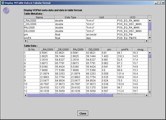
Display Data
The VOTable data used to plot the graph can be displayed in tabular format. It also displays the filters and data sets that are user-defined.
Displaying the VOTable Data in Tabular Format:
To view the VOTable data, click on "Data in Table format" submenu from the "View" menu. The "Display Data" dialog box will open.
The data is displayed in two different tables. The first table displays the field metadata of the VOTable, while the second table displays the actual data.
If points are not selected on the plot, the entire plot data is displayed.
Sample dialog box
displaying the selected data and metadata of the VOTable is shown in Figure 12.
Figure 12
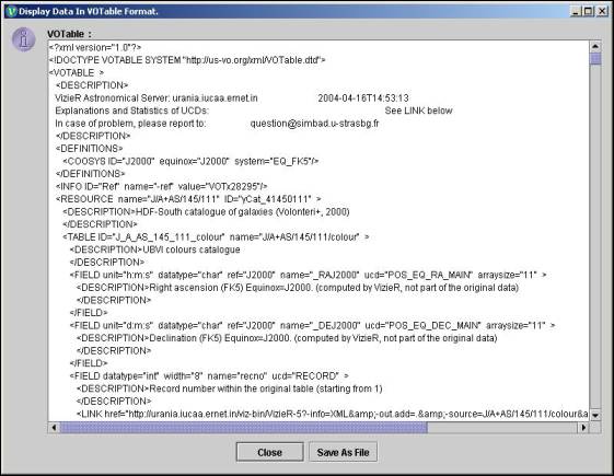
Display VOTable
Used to display Plot data in VOTable format. It also displays the filters and data sets that are user-defined.
Displaying the VOTable:
To view the VOTable, click on "Data in VOTable format" submenu from the "View" menu. The "Display VOTable" dialog box will open.
Sample dialog box displaying VOTable containing data of selected points is shown in Figure 13 below.
Figure 13
Save VOTable:
This feature is available only in the desktop version of VOPlot. To save a VOTable, click on "Save As File" button on the dialog box. The save as dialog box will appear. Select a file and click on OK. The file is saved as an XML file, VOTable format. The various user-defined filters and data columns pertaining to all points (more than 100) are saved in the file.
Note: This feature is not
available in the web-based version of VOPlot.
Feedback Address
We would be happy to receive any feedback/comments on 3D VOPlot. For feedback and comments please contact voindia@vo.iucaa.ernet.in.