3D Plots

Scatter Plot

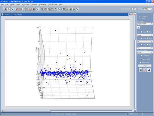
To draw a 3D plot of three different columns,

1. Select the column to be plotted on the X-axis in ``X: '' labeled combobox.
2. Select the column to be plotted on the Y-axis in ``Y: '' labeled combobox.
3. Select the column to be plotted on the Z-axis in ``Z: '' labeled combobox.
4. Click on ``3D Scatter Plot'' icon of the toolbar.

You can see the 3D scatter plot. If required, user can apply log and reversed axis functionality as described in ``Plot Functionalities -> Log'' & ``Plot Functionalities -> Reverse''.

Figure 1: 3D Scatter Plot

Overlay:
This part is described in ``Overlay'' section under ``Plot Functionalities''' ``Common to All Plots''.

Histogram

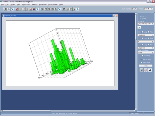
To draw the histogram of one column against another,

1. Select the column on X-axis.
2. Select the column on Z-axis.
3. Click on ``3D Histogram'' icon of the toolbar.

A sample histogram is shown in Figure 2.

Figure 2: 3D Histogram

If required, user can apply log and reversed axis functionality as described in ``Plot Functionalities -> Log'' & ``Plot Functionalities -> Reverse''.

Overlay:
This part is described in ``Overlay'' section under ``Plot Functionalities''' ``Common to All Plots''.

Surface Plot

Surface can be made using an equation or by loading a file which has regular grid data. If the surface is being made from a data file, then user can choose between Bi-Linear and Bi-Cubic Spline interpolation.

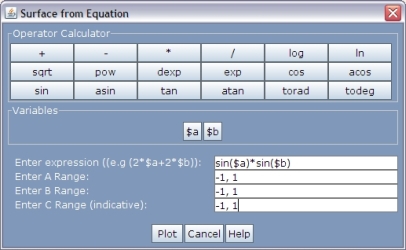
To draw the surface using an equation

1. Click on the ``Surface Plot'' icon of the toolbar.
2. Click the Equation icon in the toolbar of the Surface Plot Dialog. This launches an equation maker dialog.
3. Enter the equation in the equation maker dialog. We use $a and $b as variables. Eg: sin($a)*sin($b)
4. Then enter the ranges for a, b & c. The range for ''c'' is indicative. The actual range may differ. User has to play around with the Y range a little bit using the PlotProperties dialog (launched by clicking on the toolbar of Surface Plot dialog) after the surface is drawn
   While variables a,b make the XZ plane, c defines the height of surface at an (a,b) on the Y-Axis
5. Click Plot button to draw the surface.

Shown below is the Equation maker dialog

Figure 3: Equation Maker

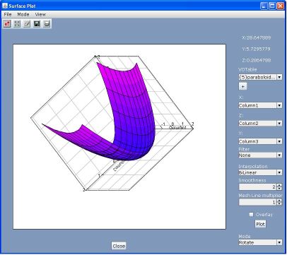
To draw a surface plot using a data file,

1. load the data file. The file should have atleast three columns (say a, b, c) in row-by-row format as shown below
   a1, b1, c11
   a1, b2, c12
   a1, b3, c13
   ...
   a2, b1, c21
   a2, b2, c22
   a2, b3, c23
   ...
   

2. click on the ``Surface Plot'' icon of the toolbar.
3. In the surface plot, the base plane is XZ plane and height axis is the Y-Axis. (For convenience the combo (drop down) boxes are ordered X, Z, Y).
   Select the columns in X and Z axis comboboxes. (In the example given in point#1 (a,b,c) map to (x, z, y))
4. Then selectc the Y-Axis combo box.
5. To determine the Y value for a particular (X,Z) we interpolate the Y values of near by (X,Z) points from the data file. User can choose betweenm BiLinear or BiCubic Spline interpolation from the Interpolation combo box.
6. Clicking ``Plot'' button draws the surface plot.
7. You can use the MeshLine multiplier combo boxes to change the number of mesh lines to be drawn. Value can vary from 0.1 to 1 insteps of 0.1
8. You can use the Smoothness combo boxes to smoothen the surface. Value can vary from 1 to 2 in steps of 0.1. Higher the value the surface is more smooth and the time taken to render the surface is more.

A sample surface plot is shown in Figure 4.

Figure 4: Surface Plot

Setting ``Smoothness'' changes the number of block counts on X axis, while ``Mesh Line multiplier'' represents number of blocks on Y axis. The smoothness or mesh line multiplier values can be set in the range between 0-2.


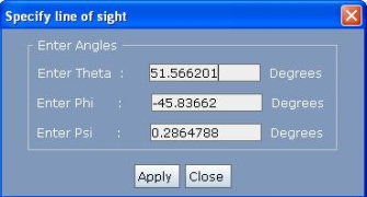
Enter line of sight in Plot:
You can set the line of sight of all the three axis by clicking of ``Enter Line of Sight'' sub menu of ``View'' menu. Clicking on this sub menu prompts up a dialog which shows three angles Theta, Phi and Psi. Theta, Phi and Psi are angles from the line of sight to the X, Y and Z axis respectively. Changing their values and clicking on ``Apply'' applies changes to the cubic grid of plot.

The Enter Line of Sight dialog is shown below in figure 5 given above.

Figure 5: Enter Line of Sight